Daline


Get Data. Find Methods. Linearize Models.

Free to use. Quick to deploy. Easy to code.
For data-driven power flow linearization and more.

model = daline.all('case118')
data = daline.generate('case.name', 'case118')
opt = daline.setopt('noise.SNR_dB', 45)
data = daline.noise(data, opt)
data = daline.outlier(data, 'outlier.switchTrain', 1, 'outlier.percentage', 2.5)
data = daline.denoise(data, 'filNoi.switchTrain', 1, 'filNoi.useARModel', false)
opt = daline.setopt('filNoi.useARModel', false, 'filNoi.zeroInitial', 0)
data = daline.deoutlier(data, opt)
data = daline.normalize(data, 'norm.switch', 1)
data = daline.data('num.trainSample', 500, 'num.testSample', 300)
opt = daline.setopt('data.baseType', 'TimeSeriesRand', 'method.name', 'RR')
data = daline.data('data.program', 'acpf', 'data.baseType', 'TimeSeriesRand')
model = daline.all('case118', 'method.name', 'RR')
data = daline.generate('case.name', 'case118')
data = daline.data('case.name', 'case39')
time_list = daline.time(data, {'LS', 'LS_SVD', 'RR'}, 'PLOT.repeat', 5, 'PLOT.style', 'light')
opt = daline.setopt('method.name', 'LS_PIN', 'variable.predictor', {'P', 'Q'}, 'variable.response', {'PF'})
model = daline.fit(data, opt)
opt = daline.setopt('method.name', 'LS_SVD', 'variable.response', {'PF'})
model = daline.fit(data, opt)
model = daline.fit(data, 'method.name', 'LS_COD')
model = daline.rank(data, method, opt)
opt = daline.setopt('data.program', 'acpf')
data = daline.data(opt)
model = daline.all('case118', 'method.name', 'RR')
data = daline.generate('data.baseType', 'TimeSeriesRand')
model = daline.fit(data, opt)
model = daline.fit(data, 'method.name', 'LS_COD')
model = daline.fit(data, 'method.name', 'LS_HBLE', 'HBL.language', 'yalmip', 'HBL.solver', 'quadprog', 'HBL.programType', 'whole')
model = daline.fit(data, 'method.name', 'LS_LIFX', 'variable.liftType', 'polyharmonic', 'variable.liftK', 2)
model = daline.fit(data, 'method.name', 'LS_WEI')
model = daline.fit(data, 'method.name', 'DRC_XYM', 'DRC.probThreshold', 90, 'DRC.gamma2', 0.5, 'DRC.language', 'cvx', 'DRC.solverM', 'Mosek', 'DRC.programType', 'whole')
model = daline.fit(data, 'method.name', 'LS_REC', 'LSR.recursivePercentage', 30, 'LSR.initializeP', 0)
model = daline.fit(data, 'method.name', 'LS_REP', 'LSR.recursivePercentage', 75)
model = daline.rank(data, {'DLPF_C', 'RR', 'PLS_REC'}, 'RR.lambdaInterval', 1e-5, 'RR.cvNumFold', 4, 'PLS.recursivePercentage', 40)
time_list = daline.time(data, {'LS', 'LS_SVD', 'RR'})
model = daline.fit(data, 'method.name', 'LS_PIN')
model = daline.fit(data, opt)
model = daline.fit(data, 'method.name', 'LS_COD')
model = daline.fit(data, 'method.name', 'LS_HBLE')
model = daline.fit(data, 'method.name', 'LS_LIFX')
model = daline.fit(data, 'method.name', 'LS_WEI')
model = daline.fit(dataN, 'method.name', 'DRC_XYM')
model = daline.fit(data, 'method.name', 'LS_REC')
model = daline.fit(data, 'method.name', 'LS_REP')
model = daline.rank(data, {'DLPF_C', 'RR', 'PLS_REC'})
time_list = daline.time(data, {'LS', 'LS_SVD', 'RR'})
model = daline.fit(data, 'method.name', 'LS_PIN')
model = daline.fit(data, 'method.name', 'LS_SVD')
model = daline.fit(data, 'method.name', 'LS_COD')
data = daline.data('case.name', 'case39')
opt = daline.setopt('variable.predictor', {'P', 'Q'}, 'variable.response', {'PF', 'Vm'})
daline.rank(data, methods)
daline.rank(data, methods, 'PLOT.response', {'Vm', 'PF'})
daline.rank(data, {'TAY', 'QR'}, 'PLOT.theme', 'commercial', 'PLOT.style', 'light')
daline.time(data, methods)
daline.time(datalist, methods)
data = daline.data('case.name', 'case39')
opt = daline.setopt('variable.predictor', {'P', 'Q'}, 'variable.response', {'PF', 'Vm'}, 'PLOT.repeat', 5, 'PLOT.style', 'light')
time_list = daline.time(data, 'LS', 'LS_SVD', 'RR', opt)
opt = daline.setopt('method.name', 'LS_PIN', 'variable.predictor', {'P', 'Q'}, 'variable.response', {'PF'})
model = daline.fit(data, opt)
opt = daline.setopt('method.name', 'LS_SVD', 'variable.predictor', {'P', 'Q'}, 'variable.response', {'PF'})
model = daline.fit(data, opt)
opt = daline.setopt('method.name', 'LS_COD', 'variable.predictor', {'P', 'Q'}, 'variable.response', {'PF'})
model = daline.fit(data, opt)
model = daline.rank(data, method, opt)
data = daline.generate('case.name', 'case118', 'data.program', 'acpf', 'data.baseType', 'TimeSeriesRand')
opt = daline.setopt('noise.switchTrain', 1, 'noise.switchTest', 1, 'noise.SNR_dB', 45)
data = daline.noise(data, opt)
data = daline.outlier(data, 'outlier.switchTrain', 1, 'outlier.percentage', 2.5)
data = daline.denoise(data, 'filNoi.switchTrain', 1, 'filNoi.useARModel', false)
opt = daline.setopt('filNoi.switchTrain', 1, 'filNoi.useARModel', false, 'filNoi.zeroInitial', 0)
data = daline.deoutlier(data, opt)
data = daline.normalize(data, 'norm.switch', 1)
data = daline.data('case.name', 'case118', 'num.trainSample', 500, 'num.testSample', 300, 'data.program', 'acpf', 'data.baseType', 'TimeSeries', 'noise.switchTrain', 1, 'outlier.switchTrain', 1, 'norm.switch', 1)
opt = daline.setopt('data.baseType', 'TimeSeries', 'method.name', 'RR')
data = daline.data('case.name', 'case118', 'data.program', 'acpf', 'data.baseType', 'TimeSeries')
opt = daline.setopt('case.name', 'case57', 'data.program', 'acpf', 'data.baseType', 'TimeSeries'); data = daline.data(opt)
model = daline.all('case118', 'data.baseType', 'Random', 'method.name', 'RR')


Utilize or compare over 55 linearization methods using one line of code in Daline

Description of the image


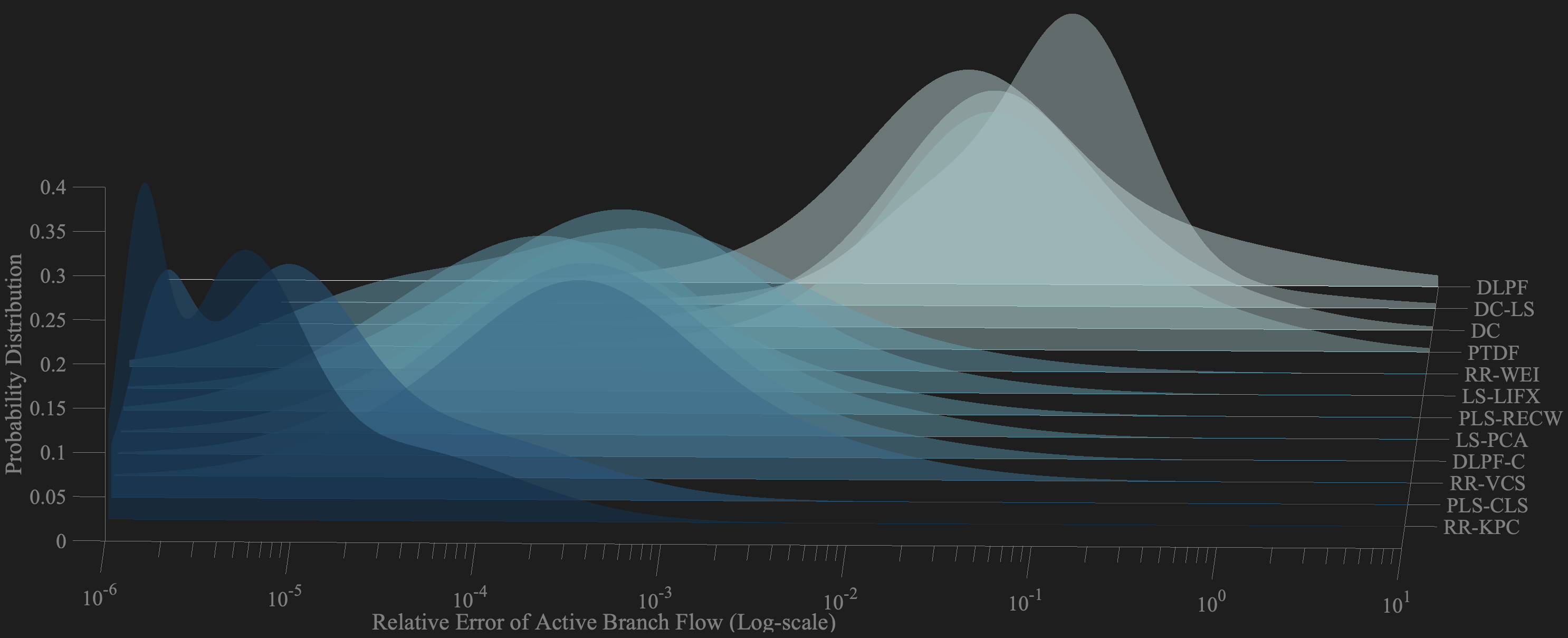
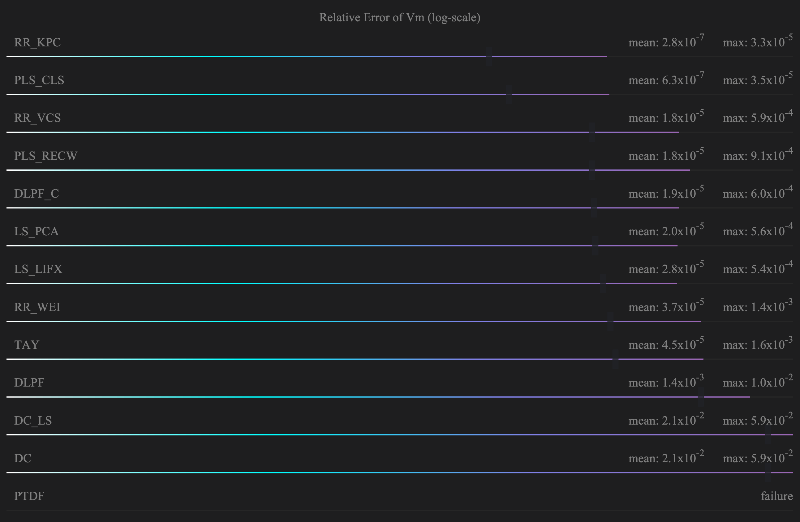
Get accuracy ranking for any states of any methods by a simple Daline command

Description of the image


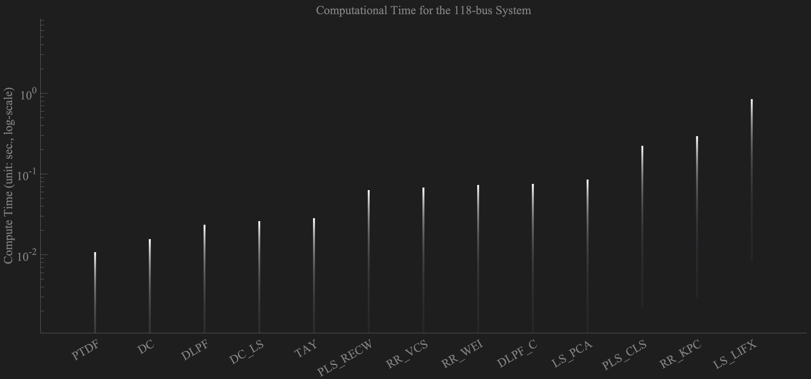
One simple command in Daline can tell you which method is faster

Description of the image


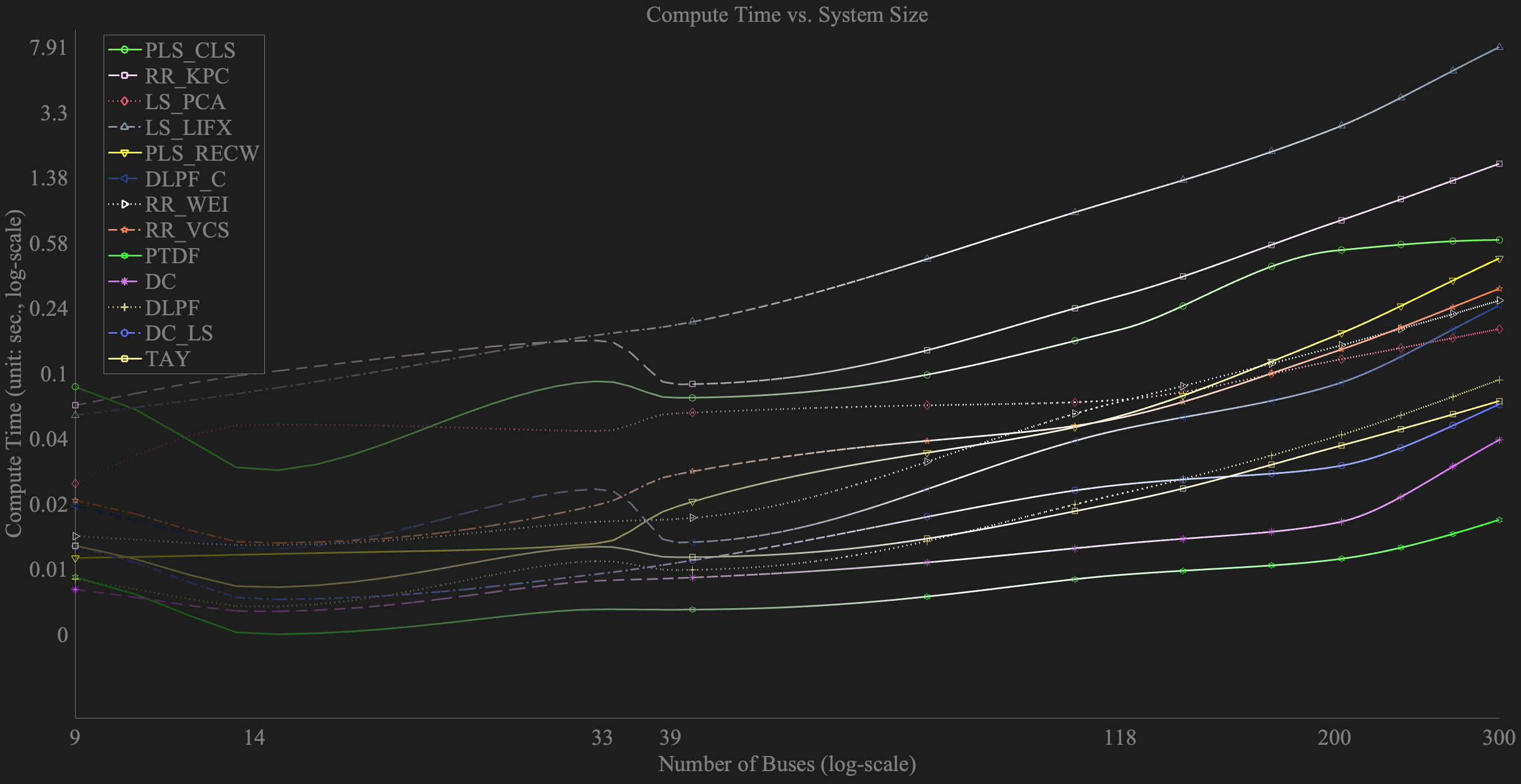
Or, tell you which method is more scalable

Description of the image


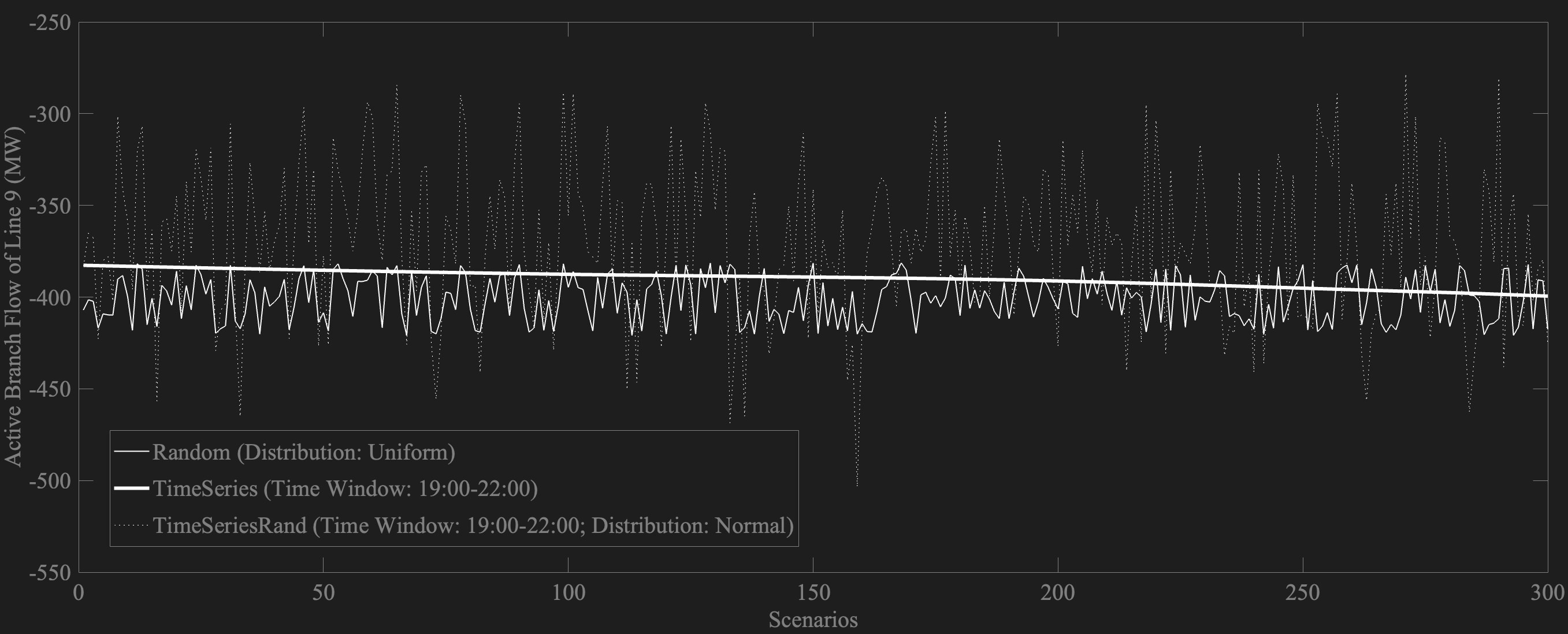
Generate, pollute, clean, and normalize (optimal) power flow data with numerous customization in one Daline command

Description of the image


Sponsors


Daline

  1. Overview

    Power flow linearization approaches should be readily accessible as fundamental tools. However, most existing methods, particularly the promising data-driven techniques, are unfortunately not open-sourced, nor available in existing toolkits or software. We thus developed Daline, a data-driven power flow linearization toolbox designed for power systems researchers, educators, and engineers. This free, open-source package consists of MATLAB-language M-files, featuring 57 linearization methods, including 53 data-driven methods and 4 commonly used physics-driven methods.

  2. Functionality

    (1) Data Generation. (2) Data Pollution. (3) Data Cleaning. (4) Data Normalization. (5) Method Selection. (6) Method Customization. (7) Model Linearization. (8) Model Evaluation. (9) Result Visualization.

Setup Daline

  1. Step 1: Download Daline

    Click daline115.zip to download the latest release version, and extract the downloaded ZIP file anywhere you like.

  2. Step 2: Install Daline

    Start MATLAB and change your working directory to the Daline directory you just extracted (the one containing daline_setup.m). Daline will be installed by typing the following command in the MATLAB command window:

     daline_setup

    The above command will install Daline with a quick test of its major functionality. If you want to install Daline while testing all its functionality, type the following command:

     daline_setup('full')
  3. Step 3: Enjoy

    There is no step 3, but you can now choose to verify all the functionality of Daline by typing:

     daline_test

    Or to verify any specific built-in linearization methods, e.g., 'PLS_REC' and 'RR_KPC', in Daline by typing:

     daline_test({'PLS_REC'; 'RR_KPC'})

    And, if you find Daline helpful for your work, please remember to cite the following reference!

    @article{Daline,
    author = {Jia, Mengshuo and Chan, Wen Yi and Hug, Gabriela},
    title = {Daline: A Data-driven Power Flow Linearization Toolbox for Power Systems Research and Education},
    journal = {ETH Research Collection}, year = {2024}, url = {https://doi.org/10.3929/ethz-b-000681867}, doi = {10.3929/ethz-b-000681867}
    }

Run Daline

  1. Quickly get a linear model

    To train a linear power flow model for the standard IEEE-118 case using the default linearization method and options, type:

    model = daline.all('case118')

    There are over 300 options/parameters to customize the behavior of the wrapper daline.all, e.g.,

    model = daline.all('case118', 'data.baseType', 'Random', 'method.name', 'LS_COD');

    Or

    opt = daline.setopt('data.baseType', 'Random', 'method.name', 'LS_COD');
    model = daline.all('case118', opt);

    The wrappers in the following examples also offer numerous options and parameters that can be adjusted using name-value pairs. These examples demonstrate only a small selection of these options to provide an easy starting point.

  2. Generate data

    To generate artificial power flow data for a user-owned MPC-structured power system using a time series loading curve, type:

    data = daline.data('case.mpc', mpc_user, 'data.baseType', 'TimeSeriesRand')

    There are more than 45 options available for customizing data generation.

  3. Train & test linear model

    To train a linear power flow model using an existing dataset with ridge regression and k-plane clustering:

    model = daline.fit(data, 'method.name', 'RR_KPC')
  4. Customize linearization methods

    To customize ridge regression with k-plane clustering, for example by enabling the auto-tuning of the regularization factor in this method:

    model = daline.fit(data, 'method.name', 'RR_KPC', 'RR.lambdaInterval', [0:1e-3:0.02])

    Ridge regression with k-plane clustering has 9 hyperparameters/options for customization in Daline.

  5. Accuracy Comparison & Visualization

    To compare and visualize the linearization error distributions of various data-driven and physics-driven approaches:

    models = daline.rank(data, {'PLS_SIM', 'RR', 'LS_COD', 'DC', 'TAY'});

    The comparison settings and the parameters for the methods can all be adjusted using daline.rank.

  6. Efficiency Comparison & Visualization

    To compare and visualize the computational efficiency of various data-driven and physics-driven approaches:

    time = daline.time(data, {'PLS_SIM', 'RR', 'LS_COD', 'DC', 'TAY'} , 'PLOT.repeat', 5);

    The comparison settings and the parameters for the methods can all be adjusted using daline.time.


More can be found in the Daline user manual.


Important Notice

1. Daline is free of charge to use and is openly distributed.

2. Daline is distributed under the 3-Clause BSD License.

3. The copyright of Daline is owned by Mengshuo Jia and Gabriela Hug with all rights reserved.

4. Daline must be cited via the following reference when used in a published work.

@article{Daline,
author = {Jia, Mengshuo and Chan, Wen Yi and Hug, Gabriela},
title = {Daline: A Data-driven Power Flow Linearization Toolbox for Power Systems Research and Education},
journal = {ETH Research Collection}, year = {2024}, url = {https://doi.org/10.3929/ethz-b-000681867}, doi = {10.3929/ethz-b-000681867}
}


Images are generated by Generative AI and may contain typos.


  • License


    Starting from version 1.1.5, Daline is distributed under the 3-Clause BSD License. Copyright (c) 2024. Primary Developers to Daline. All rights reserved.


    Redistribution and use in source and binary forms, with or without modification, are permitted provided that the following conditions are met:

    1. Redistributions of source code must retain the above copyright notice, this list of conditions and the following disclaimer.

    2. Redistributions in binary form must reproduce the above copyright notice, this list of conditions and the following disclaimer in the documentation and/or other materials provided with the distribution.

    3. Neither the name of the copyright holder nor the names of its contributors may be used to endorse or promote products derived from this software without specific prior written permission.

    THIS SOFTWARE IS PROVIDED BY THE COPYRIGHT HOLDERS AND CONTRIBUTORS "AS IS" AND ANY EXPRESS OR IMPLIED WARRANTIES,INCLUDING, BUT NOT LIMITED TO, THE IMPLIED WARRANTIES OF MERCHANTABILITY AND FITNESS FOR A PARTICULAR PURPOSE ARE DISCLAIMED. IN NO EVENT SHALL THE COPYRIGHT HOLDER OR CONTRIBUTORS BE LIABLE FOR ANY DIRECT, INDIRECT, INCIDENTAL,SPECIAL, EXEMPLARY, OR CONSEQUENTIAL DAMAGES (INCLUDING, BUT NOT LIMITED TO, PROCUREMENT OF SUBSTITUTE GOODS OR SERVICES; LOSS OF USE,DATA, OR PROFITS; OR BUSINESS INTERRUPTION) HOWEVER CAUSED AND ON ANY THEORY OF LIABILITY, WHETHER IN CONTRACT, STRICT LIABILITY, OR TORT (INCLUDING NEGLIGENCE OR OTHERWISE) ARISING IN ANY WAY OUT OF THE USE OF THIS SOFTWARE, EVEN IF ADVISED OF THE POSSIBILITY OF SUCH DAMAGE.


  • Important Notice


    The data generation functionality of Daline is built on MATPOWER, and the built-in optimization methods of Daline utilize toolboxes CVX and YALMIP. To minimize installation and setup costs, Daline includes redistributed versions of these toolboxes, in strict compliance with their redistribution licenses. License files for these toolboxes are also included in Daline . Therefore, if users redistribute Daline , they must adhere not only to Daline’s license but also to the licenses of these included toolboxes.


Please check here for the Github site

Contact Form